

(Tidy Tuesday is a project to supply weekly data sets for R users to practice their coding skills on. You can find full details here.)
It’s been a while since I took part in a Tidy Tuesday, but having not played with any R code for a while I got the urge to create some utterly pointless plots this weekend, so here we are. This week’s dataset is looking at world records in Mario Kart 64, which despite being over two decades old (don’t let it set in), is still active in the videogame speedrunning community.
First up, a ridgeline plot of the density of world record activity per track over the years:
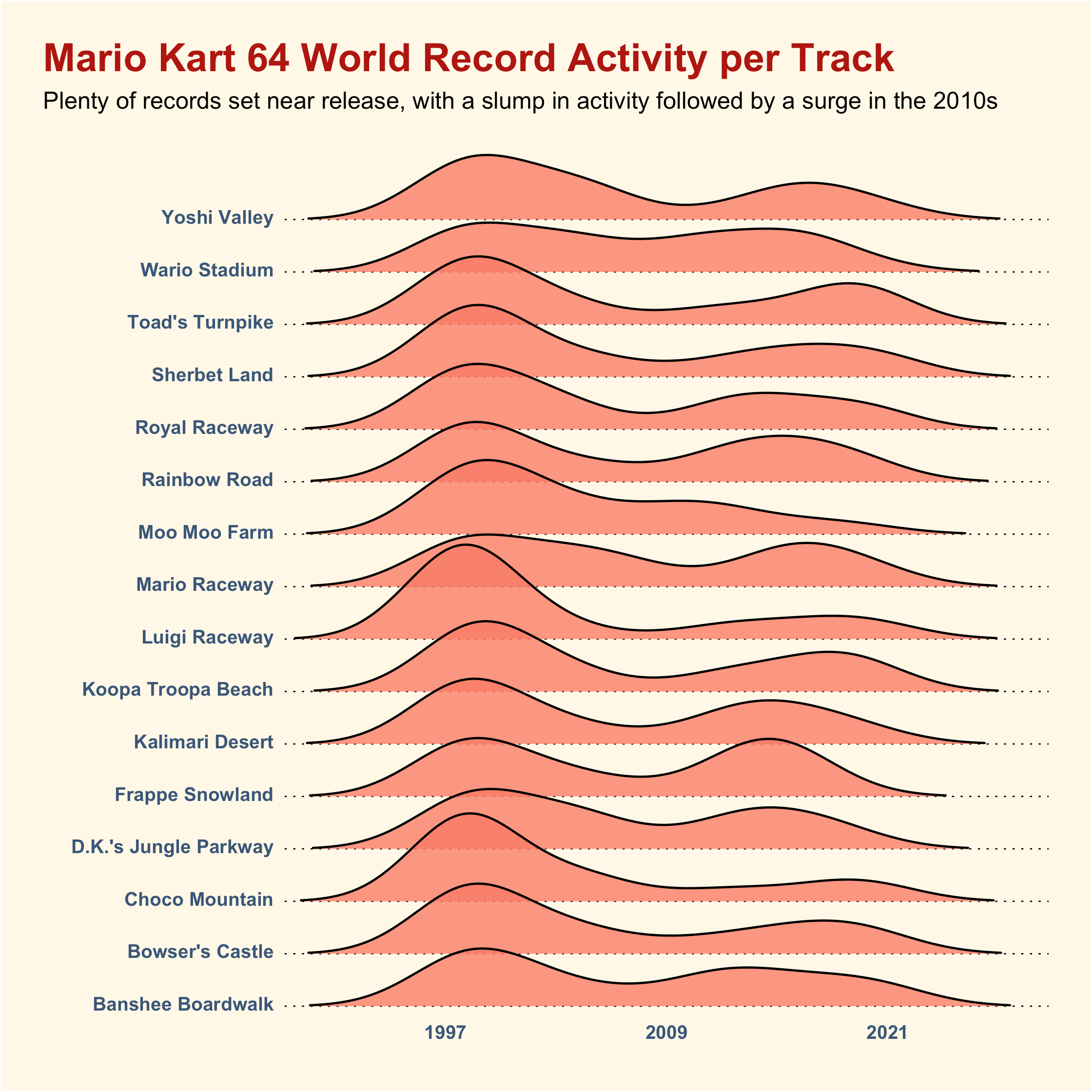
I’d seen ridgeplots quite a lot when browsing #TidyTuesday on Twitter so I figured it was about time I gave one a shot myself. I used the ggridges package and it was fun to finally have an excuse to try it out! Looking at the plot, it seems like there was a resurgence in world record activity later in the games life - most likely due to more widespread internet access and the growth of the speedrunning scene in general as a result, I imagine.
Second, a plot showing the total amount of time it would take you to complete all the tracks in Mario Kart 64 at the fastest world record pace each year:
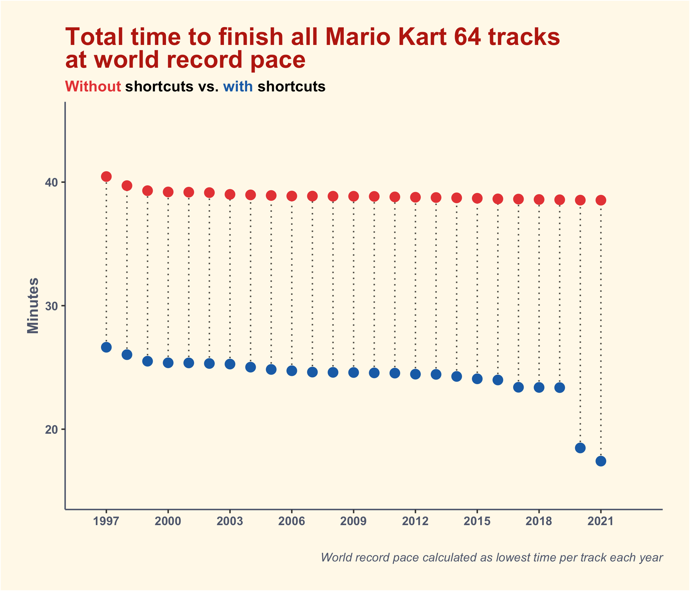
The plot itself isn’t the most interesting result (although what happened with shortcuts in 2020? My brief research reveals the possible discovery of a new technique - maybe it made all the difference!) But, the method to get the fastest time per year for both shortcut and non-shortcut uses was a fun puzzle to solve, and involved some fancy pivoting back and forth alongside the use of tidyr’s fill function to flesh out those years where no records were set. See the code for all the steps.
Speaking of the code, have you noticed the new native R pipe operator? I thought I’d give it a whirl. |> is certainly easier and quicker to type than the old %>% one, although there are one or two bits of functionality missing that mean %>% probably isn’t going away entirely just yet.
Code (also on GitHub):
library(tidyverse)
library(ggtext)
library(ggridges)

# importing data

tuesdata <- tidytuesdayR::tt_load(2021, week = 22)

drivers <- tuesdata$drivers
records <- tuesdata$records

# activity plot

records |>
  separate(date, into = c("year", "month", "day"), sep = "-") |>
  filter(shortcut == "No") |>
  ggplot(aes(x = year, y = track, group = track)) +
  geom_density_ridges(rel_min_height = 0.01, fill = "#F97B64", alpha = .8) +
  labs(x = "", y = "", title = "Mario Kart 64 World Record Activity per Track",
       subtitle = "Plenty of records set near release, with a slump in activity followed by a surge in the 2010s") +
  scale_x_discrete(breaks = c(1997, 2009, 2021)) +
  scale_y_discrete(expand = expansion(mult = c(0.01, .12))) +
  theme(legend.position = "none",
        axis.text.x = element_text(face = "bold", colour = "#3A5678"),
        axis.text.y = element_text(vjust = 0.3, face = "bold", colour = "#3A5678"),
        axis.ticks = element_blank(),
        axis.line = element_blank(),
        panel.grid = element_blank(),
        panel.grid.major.y = element_line(size = 0.3, colour = "black", linetype = 3),
        plot.title.position = "plot",
        plot.title = element_text(face = "bold", colour = "#AE030E", size = 18),
        plot.background = element_rect(fill = "#FFF8E7"),
        panel.background = element_rect(fill = "#FFF8E7"),
        plot.margin = margin(20,20,10,20))

# calculating the total times per year

all <- records |>
  separate(date, into = c("year", "month", "day"), sep = "-") |>
  filter(type == "Three Lap") |>
  expand(year, track, shortcut)

fastest <- records |>
  separate(date, into = c("year", "month", "day"), sep = "-") |>
  filter(type == "Three Lap") |>
  group_by(year, track, shortcut) |>
  summarise(min = min(time)) |>
  ungroup()

total_times <- all |>
  left_join(fastest) |>
  pivot_wider(names_from = c("track", "shortcut"), values_from = "min") |>
  fill(where(is.double), .direction = "down") |>
  pivot_longer(-1) |>
  fill(where(is.double), .direction = "down") |>
  separate(col = "name", into = c("track", "shortcut"), sep = "_") |>
  group_by(year, shortcut) |>
  summarise(total_time = sum(value)) |>
  ungroup() |>
  mutate(shortcut = factor(shortcut))

# total times plot

total_times |>
  pivot_wider(names_from = "shortcut", values_from = "total_time") %>%
  ggplot(aes(x = year)) +
  geom_linerange(aes(ymin = Yes/60, ymax = No/60), colour = "#4C4A42", linetype = 3) +
  geom_point(aes(y = No/60), size = 3, colour = "#E03135") +
  geom_point(aes(y = Yes/60), size = 3, colour = "#185AA6") +
  labs(x = "", y = "Minutes",
       title = "Total time to finish all Mario Kart 64 tracks<br>at world record pace",
       subtitle = "<span style = 'color:#E03135;'>Without</span> shortcuts vs. <span style = 'color:#185AA6;'>with</span> shortcuts",
       caption = "World record pace calculated as lowest time per track each year") +
  expand_limits(x = c(-1, 28), y = c(15, 45)) +
  scale_x_discrete(breaks = seq(1997, 2021, by = 3)) +
  theme(legend.position = "none",
        axis.text.x = element_text(face = "bold", colour = "#4D556B"),
        axis.text.y = element_text(face = "bold", colour = "#4D556B"),
        axis.title.y = element_text(face = "bold", colour = "#4D556B"),
        axis.line = element_line(colour = "#4D556B"),
        panel.grid = element_blank(),
        plot.title = element_textbox(face = "bold", colour = "#AE030E", size = 18),
        plot.background = element_rect(fill = "#FFF8E7"),
        panel.background = element_rect(fill = "#FFF8E7"),
        plot.margin = margin(20,20,20,20),
        plot.subtitle = element_textbox(face = "bold"),
        plot.caption = element_textbox(face = "italic", colour = "#4D556B"))
