Scrivdown

In my last post on Bookdown, I mentioned using writing environments other than RStudio to work on non-code text sections. As I recommended in that post, I’ve been using iA Writer as my main text editor. It’s a great plain editor - I’m using it to write this post now. But, as my last big writing project got bigger, and bigger ¹, I found myself missing a lot of the writing project management tools from my previous preferred writing app - Scrivener.

In particular, I missed the ability to segment my work into an outline structure. I initially tried having separate plain text files to break up the text into sections to work on, but although Bookdown would stitch these back together into one final piece fine, they weren’t easy to work with. In particular, Bookdown reassembles these files in the order they are listed in the directory, so I ended up numbering all my files (01-intro.Rmd, 02-litreview.Rmd, 03-method.Rmd, etc). But, in Scrivener I would often work as small as the paragraph level, dragging and dropping chunks of text around to see what flowed best in the overall document. This just wasn’t practical in plain text files, as I’d have to re-number everything if I wanted to insert something between two existing files, or just live with cutting and pasting paragraphs within docs. Not the end of the world, but just not as easy as Scrivener.

So I wanted to move back to Scrivener, but I wanted to keep all the benefits of Bookdown - namely, having my R code included in the document to produce plots/tables, rather than importing images or copying/pasting tables into Scrivener each time I iterated on my code. I also wanted to keep the benefits of compiling to PDF with LaTeX, like auto-generated tables of contents and lists of figures/tables.

I basically wanted to use Scrivener as my plain text editor. And it turns out, that’s actually pretty easy, but not necessarily straightforward. Here’s how I set it up.

Inspiration

The idea for this workflow was heavily inspired by Scrivomatic, by Ian Max Andolina. Scrivomatic is great, and I used it extensively in the past, but it doesn’t deal with R code. This is the main difference to my setup; the additional layer of R and Bookdown, which also results in a simpler Scrivener setup as things like front-matter yaml code remain in Bookdown itself.

There are some other useful hints in the Scrivomatic docs worth looking at, like this tip on using custom styles when exporting to Word. It’s definitely worth checking Scrivomatic out if you like the idea of this kind of workflow and don’t need the additional step of including R code when compiling your document.

Scrivener setup

The nice thing about Scrivener is that you can set up your writing preferences in it, then tell Scrivener how much of that to keep or discard when it comes time to export your document to the final file format. So, you can set up your internal Scrivener editor pretty much as you like - fonts, colours, styles, whatever makes writing easiest for you. As we’re compiling to plain text, all that will be stripped out of the final export, but it can be useful for editing (I like to highlight bits I need to work on, for example).

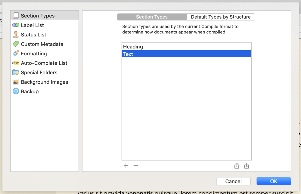
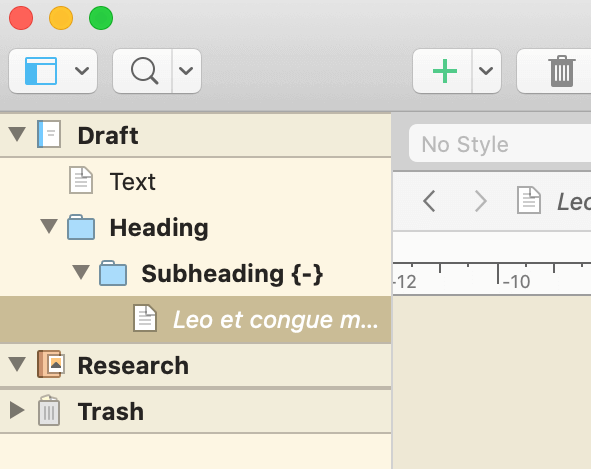
The main thing you need for your project is in the menu Project > Project Settings... > Section Types. Here, I suggest just having Heading and Text sections setup, and under Default Types by Structure, setting all folders to Heading and files to Text. Then, you can setup your project in your binder with folders for each heading, nested folders for sub-headings, and files within these containing your actual text.

Because Scrivener can auto-detect heading levels from the Binder structure, then top-level folders will be H1s (# Heading), sub-folders will be H2s (## Heading), and so on.

Then, in the File > Compile menu, set the Compile for dropdown at the top to MultiMarkdown. You should set up your own custom compile format - in the left of the window, right-click Basic MultiMarkdown and choose Duplicate & Edit Format. This will open the compile format editing menu ². Give your new format a name, and choose to save it either into the project - so it will travel around with the actual .scriv file you’re working on - or globally, so it will be available in Scrivener no matter which project you open. I like to save a generic global version, then duplicate that into each project that I can fine-tune to that individual project if required.

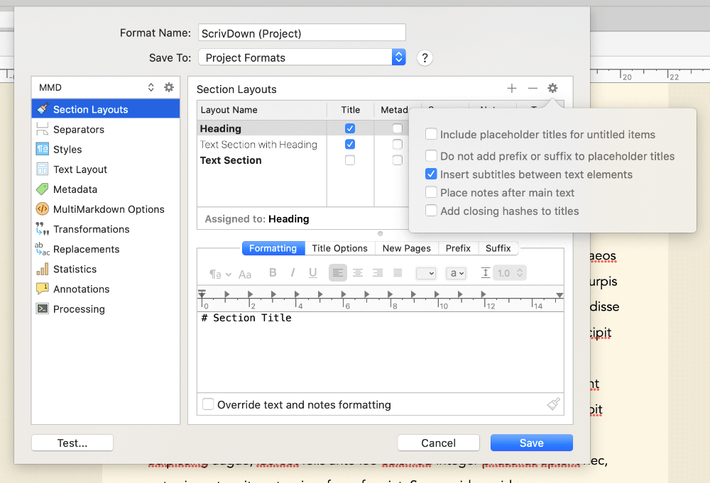
In the format editor, click Section Layouts, then click the little gear settings icon in the top right. Make sure to untick Add closing hashes to titles. By default, Scrivener puts markdown headings as # Heading #, and this option will turn them into just # Heading. This allows you to put additional Bookdown header options, like {-} to create an unnumbered heading, in your folder names/headings.

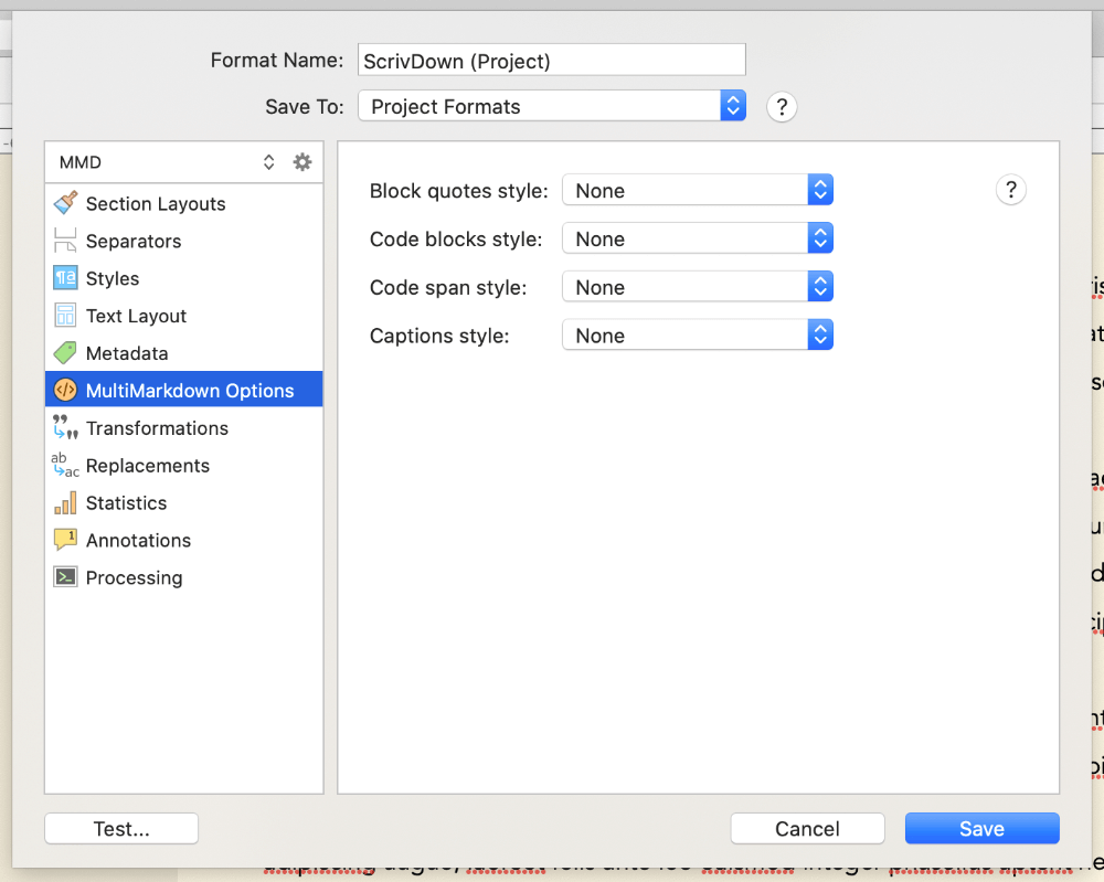
If you like to use styles in your Scrivener editor while writing, then while still in the format editor, click MultiMarkdown Options, then set all the dropdown options here to None. This stops Scrivener from formatting our output based on internal Scrivener styles you might use - for example, by default it indents any text marked with the Code block style in the output. I found it easier to just switch these off, but you can experiment with them if you like.

You can play with some of the other settings in the compile format editor too. Most of it is fine as default, but you might like to explore it more. Make a note of the Processing section - we’ll come back to this later. Otherwise, just click Save to save your new compile format.

Back in the compile menu, you can make sure all the headings/text you want to compile are selected on the right, and that they’ve all been assigned the correct section layout. If you get a yellow box in the middle saying your layouts haven’t been assigned to a section type, just click Assign Section Layouts at the bottom and make sure Heading is set to Heading, and Text is set to Text Section.

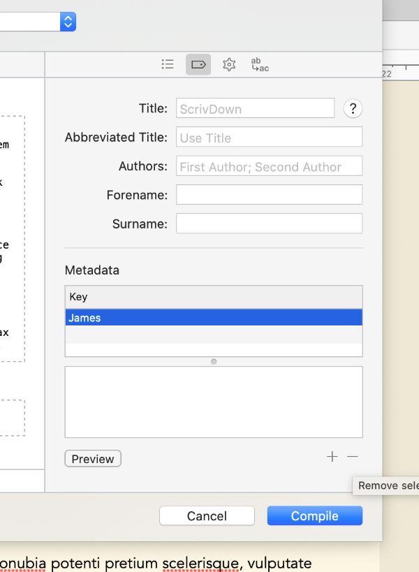
Click the little tag icon in the top right of the compile menu, and delete any metadata fields listed here by clicking the row in the key box, then clicking the minus sign at the bottom of the menu. If the default metadata is left in, Scrivener will insert it as yaml at the top of the exported file. It won’t break anything, but as we’re using Bookdown for all our metadata, it’s unnecessary to include it again.

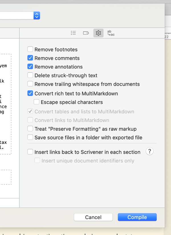
Finally, click the cog icon in the top right of the compile menu, and tick Convert rich text to MultiMarkdown. This lets you use visual WYSIWYG styling like italics and bold in the editor, and Scrivener will automatically put markdown formatting around it on export. Then, untick Escape special characters, otherwise Scrivener will escape out the code chunks we write later. The other options here can remain as default, but you can experiment with them if you feel confident.

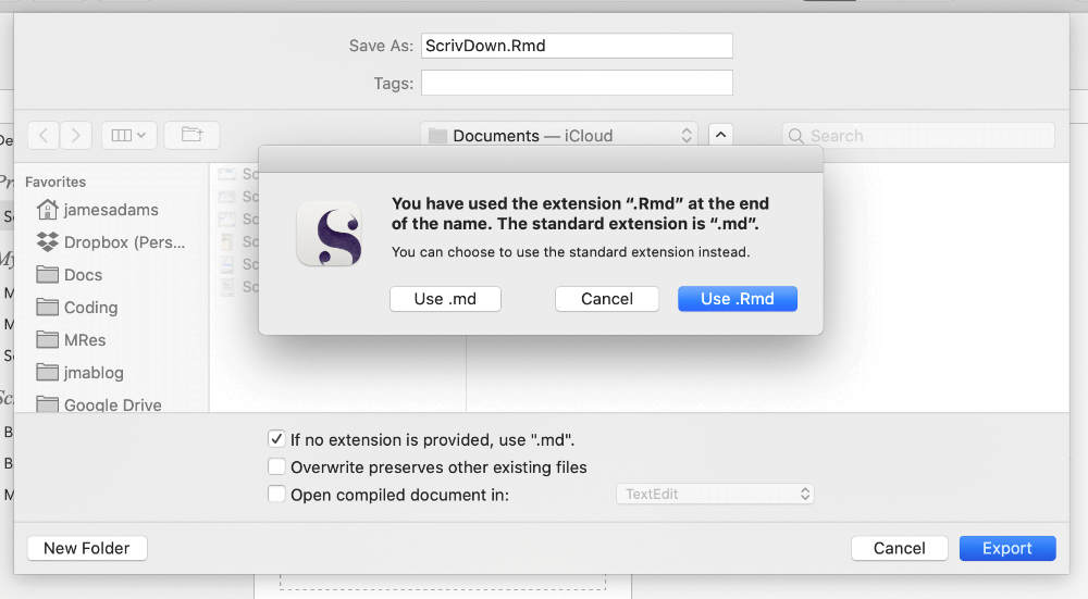
And that’s it for Scrivener setup - you can then click Compile to export your plain text file. Scrivener will default to file.md as a file extension, but you can actually just type file.Rmd in the save dialogue for your filename to export to .Rmd - you’ll get a pop-up warning but just click the option that lets you use a custom file extension. You can check the output looks how you want - it should basically just resemble any other Rmarkdown file, as if you’d written it straight in RStudio.

So that’s Scrivener setup - what about R and Bookdown?

R / Bookdown setup

On the R side of things, you can basically setup a Bookdown project as normal - so project creation, index.Rmd setup, _bookdown.yml and _output.yml, all that stuff, remains the same. If you’re unclear on any of that, the Bookdown manual is the best place to start.

The main thing is to make sure you’ve set up Bookdown to find the file you’re exporting from Scrivener - I usually have a subdirectory like book/src that I then direct _bookdown.yml to find with rmd_subdir = "book/src", and then export from Scrivener into that directory. There’s a bit more detail on that in the manual specifically here.

The main difference is that code isn’t going to be written directly into your Rmarkdown text in Scrivener - instead, code is written and worked on in separate .R script files. ³ I like to store mine in another directory (I use an analysis folder in the Bookdown project directory). These can be worked on in Rstudio in the normal way. But, although the code will be written in .R files, rather than .Rmd, we’re still going to divide the code up into Knitr chunks using the following syntax:

## ---- example-table

mtcars %>%
  head(3) %>%
  kable(caption = "Example table with a long caption.",
      caption.short = "Short caption.",
      booktabs = T)
      
## ---- example-plot

mtcars %>%
  ggplot(aes(drat, wt)) +
  geom_point()
  

Knitr chunks in .R files are a bit strange, and don’t look like they do in .Rmd files, but basically boil down to two hashes and at least four dashes, followed by a chunk name: ## ---- chunk-name. Make sure not to have any spaces in the chunk name. It’s a little unclear, but a chunk will basically include everything up to the next chunk header.

Anyway. You can work through your analysis in R exactly the same as usual, importing/creating data and analysing it however you see fit, then creating all your output tables/plots as chunks. For example, I can put the code above in a file called my-code.R in the analysis folder. You can split your analysis across multiple .R files too, if that’s easier. Just make sure each chunk name, even if in different .R files, is unique.

Why do it this way? You’ll see in the next step.

Linking the two

So, now we have our Scrivener setup to export to a plain text file for Bookdown to find in book/src, and our analysis code in analysis. But what if I now want to include the example-table from above in my final document?

This is where knitr::read_chunk() comes in! This function reads in an external file, without evaluating it. So, somewhere at the start of our index.Rmd file for Bookdown, we just insert a chunk with the following:

knitr::read_chunk("analysis/my-code.R")

You can do this for any .R file you want included.

Then, in Scrivener, at the point we want to insert the table, we just have to put an empty Rmarkdown code chunk, making sure it has the same chunk name as the table’s chunk in the .R file. For example:

Here is my text in Scrivener.

​```{r example-table}
```

See my table above for more.

This will come out as plain text in our Scrivener export, and then when the book is rendered with Bookdown, be evaluated as code. Basically, if a chunk is empty, knitr looks for another chunk with the same name, and runs the code within that. As we pulled in our .R file with read_chunk, Knitr instead goes and finds our example-table chunk there, and runs it at the point in our document where we included our empty code chunk. This is why every chunk needs a unique name!

We can even cross-reference these chunks the exact same way we usually cross-reference things in Bookdown, with \@ref(tab:example-table) for the above. It all just works exactly the same as regular Rmarkdown docs, we’re just inserting the chunk code from an external source.

Phew! That’s a little mind-bendy, but it means that when we update any code in our analysis, we can re-render the book with Bookdown and have the relevant code chunk automatically fetched and run within the text.

The whole workflow therefore becomes:

1. Setup Bookdown
2. Analyse data with .R files in analysis folder
3. Create any tables/plots required as knitr chunks in .R files in analysis
4. Write prose in Scrivener
5. Include empty named chunks where tables/plots are required in Scrivener prose
6. Compile from Scrivener to .Rmd in Bookdown source directory
7. Render final document with Bookdown

All the normal Bookdown options for step 7 should work fine, including my previous post about compiling to different document formats from Bookdown.

Some complications

There are a couple of caveats worth noting with this method. First, only chunks from our analysis files that we explicitly include with an empty code chunk will be run. Anything not referenced with an empty code chunk somewhere in our final .Rmd source text won’t be run. This means any setup code - for example, data creation/import/cleaning steps - in an analysis script still need to be referenced somewhere, even if they aren’t creating a table or plot to be displayed. I find the easiest way to deal with this is to just put all the setup code in one big data-setup chunk at the start of an analysis script named something like setup.R, then include an empty chunk with the same data-setup name in index.Rmd.

Secondly, if you want to set code chunk options, you need to include those on the empty chunks, rather than in the analysis code chunks. This most usefully applies to plots in my experience so far. For example, to insert the example-plot from above with some chunk options:

Here is a plot:

```{r example-plot, fig.cap="Here is the caption for my example plot.", fig.scap="Example plot"}
```

Wow! What a plot. Figure \@ref(fig:example-plot) is amazing.

Because this can get messy in Scrivener, I tend to just use individual chunk options to set plot captions as above, then set a whole load of default chunk options for plots in my setup in index.Rmd:

knitr::opts_chunk$set(echo = FALSE,
                      fig.pos = "tbp",
                      out.extra = "",
                      out.width = "100%",
                      fig.retina = 2)

Post processing

If you’d like to make things a little more efficient, we can also link steps 6 and 7 from our workflow above using Scrivener’s ability to run a processing script on our exported plain text file. ⁴

Note: The below is for getting this working on MacOS. I don’t know how it differs for other operating systems. Soz.

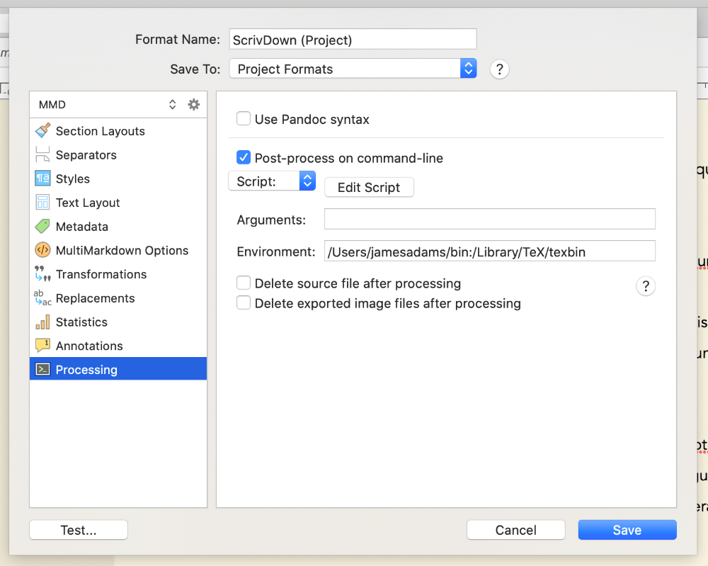
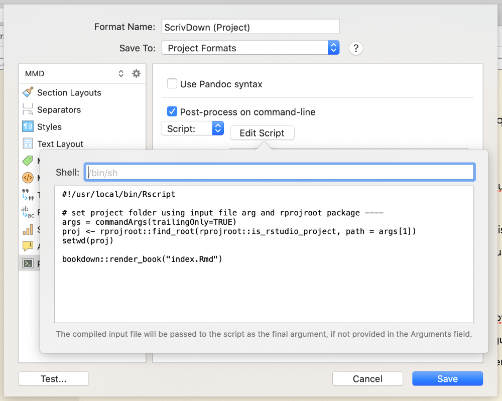
Head to File > Compile, right-click your custom format and select Edit Format, then click the Processing menu option on the left. Tick the box that says Post-process on command-line to enable the post-processing options below. Click the Edit script button now to pop-up a little window that we can put our script in.

You can run R code from the command line using the Rscript executable and linking to it at the top of your shell script - if you’ve installed R, you can find where this is installed by running which Rscript at the command-line. Mine was in /usr/local/bin/Rscript, so I entered this at the top of my script following a shebang. This lets us run regular R code in the rest of the script, that will be passed to Rscript to run.

Scrivener also provides the full file path of the exported .Rmd file to our script as a command-line argument. Using this, we can run commandArgs(trailingOnly=TRUE) to collect those args. Then, using the rprojroot package, we can run:

rprojroot::find_root(rprojroot::is_rstudio_project, path = args[1]) 

…to set our working directory to the Rstudio project directory for our Bookdown project (assuming you’re using Rstudio projects with your Bookdown setup) and then render our book! ⁵

Basically, just copy and paste this in to the Edit Script pop-up:

#!/usr/local/bin/Rscript

args <- commandArgs(trailingOnly=TRUE)
proj <- rprojroot::find_root(rprojroot::is_rstudio_project, 
				path = args[1])
setwd(proj)
bookdown::render_book("index.Rmd")

Provided all your Bookdown files are setup (metadata in index.Rmd, _bookdown.yml and _output.yml in project folder), the book should build.

You can also just set the working directory manually if you don’t want to install rprojroot:

#!/usr/local/bin/Rscript

setwd("~/path/to/project/folder")
bookdown::render_book("index.Rmd")

Just be aware this will be hard-coded into your compile format, so if you move your files, or change project, be sure to update it.

Once you’re able to set your project directory as the working directory, you can write any R code you want afterwards. For example, I use renv to manage my project libraries and have built my own custom book rendering function that I load with devtools, so my full post-processing script in Scrivener is actually this:

#!/usr/local/bin/Rscript

args <- commandArgs(trailingOnly=TRUE)
proj <- rprojroot::find_root(rprojroot::is_rstudio_project,
			path = args[1])
setwd(proj)

source("renv/activate.R")
devtools::load_all()
build_book()

I turn this post-processing on/off as I feel when I’m working - sometimes it’s easier to render the book from within Rstudio, if I’m tweaking Bookdown settings for example, and sometimes I want to iterate on my actual prose so I’ll set it to auto-render from Scrivener.

Finally, because the shell Scrivener uses is (to quote the manual) “a very limited non-interactive shell”, I found it was having trouble finding my lualatex install. The answer was to enter this in the Environment text field under the Edit Script button:

/Users/james/bin:/Library/TeX/texbin

This added my user bin folder and TeX install to the PATH environment variable for Scrivener’s shell. If you’re getting similar errors, you may need to figure out where the thing Scrivener is failing to find lives on your computer, and add that to the Environment text field. Just enter the full paths to any folders you want found, separated by a colon.

Downsides

There are a couple downsides to this workflow that are worth noting. Mainly, it’s a one-way street from Scrivener to .Rmd. If you render your final document, then notice some plot caption needs to be changed, you have to go all the way back to Scrivener and re-export to .Rmd then re-render with Bookdown. The post-processing setup above can help minimise this, but it is a little more round-the-houses than just editing and knitting directly in Rstudio. I find this trade-off worth it, as it still saves me from all the time I used to spend exporting plots as images, importing them into Scrivener, then compiling from Scrivener anyway.

Secondly, in my experience Scrivener doesn’t play all that nicely with version control systems like git. It will work, but because a .scriv project file is really just a directory of other files, there’ll be a large amount of changes per commit every time you change something in your Scrivener project. So, if GitHub or similar is your preferred way of syncing your work across devices, it might be a little inconvenient. I find it best to set my gitignore to exclude .scriv files, only track my exported .Rmd files in git, and then just sync Scrivener using Dropbox to edit on the go with the iOS app. I also use the Snapshot feature in Scrivener itself as an in-built version control, if I ever need to rewind to previous drafts of pieces of text.

I feel like these drawbacks are pretty manageable and are definitely offset by all the writing tools Scrivener provides, now paired with all the functionality of Rmarkdown/Bookdown and LaTeX.

Thanks for reading this behemoth of a post, and I hope it’s somewhat helpful to anyone looking to make use of these two amazing writing tools together. Get in touch if you’ve got any other Scrivener/Bookdown tips!